Excel Tricks

Introduction

At times, some works (especially statistics reporting) are not difficult, but just too tedious to do it. Hence, we hope all report things can be auto-calculated with each new data entry.

Here are some useful Microsoft Excel tricks that you should learn up to make it not a mission impossible.

Ctrl + Shift to Select

To quickly select a dataset, you can click in the first cell that you want to use and hold down Ctrl+Shift, then hit

Down arrow or Up arrow to get all the data below or above in the column.
Left arrow or Right arrow to get the data in the row (to the left or right respectively).

Separate Line within a Cell and Wrap Text

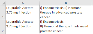
In Microsoft Excel, pressing ALT+Enter creates a new line within a cell. This just to make the data to be presented in a neater manner. An example is as below.

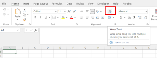
Wrap Text Option under the Home tab automatically resize the row or column so that the text re-wraps to fit.

Use AutoFilter

The AutoFilter feature is such a useful feature when dealing with spreadsheet data. We can find, show or hides values, as well as sorting the data in ascending or descending order.

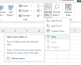
Highlight the title row of the spreadsheet data.
Go to the Home tab on the Ribbon, then Sort & Filter > Filter.

Create a Drop-down List

Frankly, there are a number of circumstances where you want your user to give only a specific value available from a certain list, for example "yes or no" or "male or female". The value selected might affect the result of the equations that we write later.

Always remember that program only do what they are being told, they will not interpret the data input and run on its own judgement.

For example, given a value of certain cell is equals to "male" or "female", the creatinine clearance equation written in another cell will run automatically and give a result. However, if the user only input "M" or "F", the result of the equation will be in an error.

To avoid this from happening, a possible solution will be to create a drop-down list, where user can only select options from a limited list.

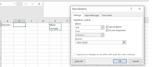
First, we will type the entries that you want to appear in your drop-down list.
Select the cell in the worksheet where you want the drop-down list.
Go to the Data tab on the Ribbon, then Data Validation.
On the Settings tab, in the Allow box, click List.
Click in the Source box, then select your list range (you just need to drag across the range of entries that you did in step 1).
Click OK.

If you are interested to learn more, you may look into dependent drop-down lists in Excel.

Input Values Starting with Zero

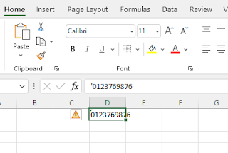
By default, Microsoft Excel will delete the zero whenever an input value starts with zero. This problem can be solved easily by adding a single quote mark ahead of the first zero, as shown.

Number Formats

In Microsoft Excel, you can format numbers in cells for things like currency, percentages, decimals, dates, time or others. It is quite self-explanatory that we would like to have the data input to be presented in a certain format.

For example, we might want the date to be presented in a "DD/MM/YYYY" or "MM/DD/YYYY" format. To avoid confusion, I would suggest using "14-Mar-2012", where it is almost unlikely for you to be confused with which number is month or date.

To set number formats in Excel:

Select a cell or a cell range
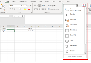
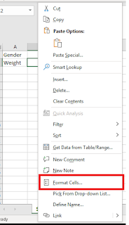
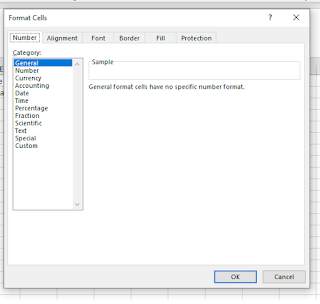
On the Home tab, select Number from drop-down; OR right-click the cell or cell range, select Format Cells....
Select the format you want and click OK.

VLOOKUP Function

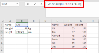
One of the key Microsoft Excel functions that you should master would be VLOOKUP function. We use VLOOKUP when we need to find things in a table or a range by row. For example, you would like to find the weight and height by your student's name.

In its simplest form, the VLOOKUP function says:

VLOOKUP(What you want to look up, where you want to look for it, The column number in the range containing the value to return, Return an Approximate or Exact match - indicated as 1/TRUE or 0/False)

The four pieces on information that you would need to build the VLOOKUP syntax:

The value you want to look up, also called the lookup value.
The range where the lookup is located (you may drag across the table to name it). Remember that the lookup value should always be in the first column in the range for VLOOKUP to work correctly.
The column number in the range that contains the return value. For example, if you specify B2:D11 as the range, you should count B as the first column, C as the second, and so on.
Optionally, you can specify TRUE if you want an approximate match or FALSE if you want an exact match of the return. If you do not specify anything, the default value will always be TRUE or approximate match.

For an example:

If you would like to learn something more, you may look into XLOOKUP function, an improved version of VLOOKUP.

IF Function

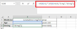
The IF function is one of the most popular functions in Microsoft Excel, and it allows you to make logical comparisons between a value and what you expect.

An IF statement can have two results:

The first result is if your comparison is True.
The second result is if your comparison is False.

For example, =if(C2="Yes",1,2)

If C2 is equal to "Yes", then it will return a "1".
However, if C2 is not equal to "Yes", then it will return a "2".

Here is my example:

Note: "" in Microsoft Excel will return an empty string.

To make things more complicated, you may use IF with AND, OR and NOT functions:

AND =if(AND(Something is True, Something else is True),Value if both True, Value if either False)
OR = if(OR(Something is True, Something else is True), Value if either True, Value if both False)
NOT = if(NOT(Something is True),Value if True, Value if False)

ROUND Function

I guess, the function itself is quite self explanatory. It allows you to round a number to a specified number of digits. When you are creating a calculator, sometimes the answer could be a number with a long list of decimal values, hence this function will be handy.

ROUND(number, num_digits)

For example, if cell A1 contains 23.7825, and you want to round that value to two decimal places, you can use the following formula:

=ROUND(A1,2)

The result of this function is 23.78.

Just a remark, there is also ROUNDUP and ROUNDDOWN function.

COUNTIFS and SUMIFS Function

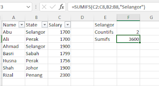
These are two functions that you may find very useful to perform auto-calculation for reporting purposes.

COUNTIFS

Applies criteria to cells across multiple ranges and counts the number of times all criteria are met.
COUNTIFS(Where you want the first criteria to be checked on, First criteria, Where you want the second criteria to be checked on, Second criteria, ...)

SUMIFS

Adds the cells in a range that meet multiple criteria.
SUMIFS(Values that you want to sum up, Where you want the first criteria to be checked on, First criteria, Where you want the second criteria to be checked on, Second criteria, ...)

NOTE: To count the number of cells that are not blank, you can either =COUNTIFS(A2:A11,"<>") or =COUNTA(A2:A11).

Dollar Sign ($) - Absolute and Relative Cell References

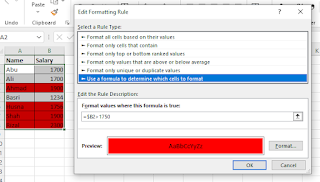
When writing an Excel formula, $ in cell references serves to tells Excel whether to change or not to change reference when the formula is copied to other cells.

Absolute and Relative Cell References in Excel

There are numerous instances where we can use this useful knowledge. The Excel functions below highlight the rows where the salary column is above 1750.

NOTE: There are also some circumstances that we may choose not to lock on any reference cells, for example comparing 2 spreadsheet data if there is any change.

Sync Data Effortless Between Google Sheets With IMPORTRANGE

IMPORTRANGE is a time-saving function that eliminates the need to copy data manually across multiple spreadsheets.

It allows for automatic synchronization of data from one Google Sheet to another.

Steps

Open the source Google Sheet containing the data you want to sync. Copy the shareable URL from the address bar.
Open the destination Google Sheet where you want the synced data to appear.
In a cell of the destination sheet, type the following formula:
=IMPORTRANGE("Source Spreadsheet URL","Source Range")
For example, =IMPORTRANGE("https://docs.google.com/spreadsheets/d/abcd12345678","Sheet1!A1:C10")

NOTE: IMPORTRANGE is specifically designed for pulling data within Google Sheets. For importing data from other file formats like .csv or .txt, use the IMPORTDATA function.

Summary

Although the tricks are taught individually, but they can be used in combination within a single cell to create numerous possibilities.

In case you need some ideas to perform a certain task, do not forget to Google it.

Search This Blog

Rx Note